This eBook discusses the impact of weather on facility energy use. It introduces two free online tools for understanding and quantifying weather effects on facility energy use—the CBECS survey database and WeatherDataDepot.com. The meaning and value of the degree day concept is also explored in detail.
This eBook is intended for energy stakeholders seeking a greater understanding of weather metrics and how they are used to enhance building energy analysis.
Quantifying Weather Impact
We are all aware that the weather affects energy consumption in a building. But to what degree? Can the weather impact be accurately quantified on a building-by-building basis? How can we know the impact of extreme and varying weather on the buildings in our property portfolio? And how can we use that knowledge to assess our energy management efforts?
It’s possible to answer these important questions with an acceptable degree of detail and precision using available quick, convenient and free online tools. This eBook will discuss several ways to measure the impact of weather on your facility energy use.
CBECS
One of the least expensive ways to obtain a basic weather assessment for a building is to obtain typical energy usage data from similar structures. This information is available through CBECS, the Commercial Building Energy Consumption Survey. CBECS is a massive database that details energy use in thousands of buildings across the United States.
According to the CBECS website, CBECS is “a national sample survey that collects information on the stock of U.S. commercial buildings, including their energy-related building characteristics and energy usage data (consumption and expenditures).”
One of those “building characteristics” is weather sensitivity.
Since the CBECS database has been made publicly available, several companies have provided online interfaces for accessing the relevant data more easily.
First, we enter basic information about a Pennsylvania office building, including:
location
square footage
building primary use
year of building constructionbenchm
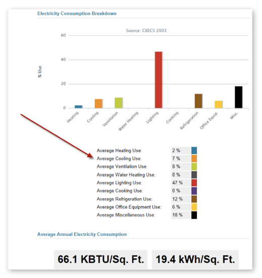
Then we can review the data returned from the CBECS database in an attractive graphical format:
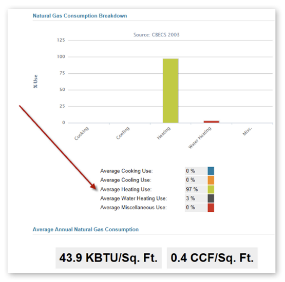
This chart provides a commodity-by-commodity evaluation of energy use. Since CBECS is comparing the office building only with similar types of buildings in similar geographical locations, we can infer that our results will be similar. In the example on the previous page, the statistical model suggests that air conditioning will consume about seven percent of the electricity required for building operation. In the example below, you can see that about 97 percent of the natural gas will be consumed by the building’s heating system.
The CBECS data suggests that this type of office building will consume 110 kBtu per square foot per year, of which 47 kBtu/SqFt will be attributable to weather. This represents 43 percent of the total energy use for the facility.
Weather Data Depot
From the CBECS survey data, we have learned that close to half of our office energy expenses may be due to weather for a building of this type in this location. But how much will that percentage vary from year to year? Will there be enough of a variation to create unanticipated budget issues? How can we analyze and quantify these variations in weather?
A very helpful free tool for historical weather analysis and forecasting is Weather Data Depot (www.WeatherDataDepot.com). Also created by EnergyCAP, Inc., this website provides weather data from The Weather Company (TWC), which is owned by IBM and hosts the popular Weather Channel.
To maintain the Weather Data Depot website, EnergyCAP processes data for more than 14,000 virtual and actual weather stations each day. The mean daily dry bulb temperature data for each location is converted to degree days and posted to the website, enabling the user to access nearly 20 years of historical temperature severity data for any specified U.S. geographical location.
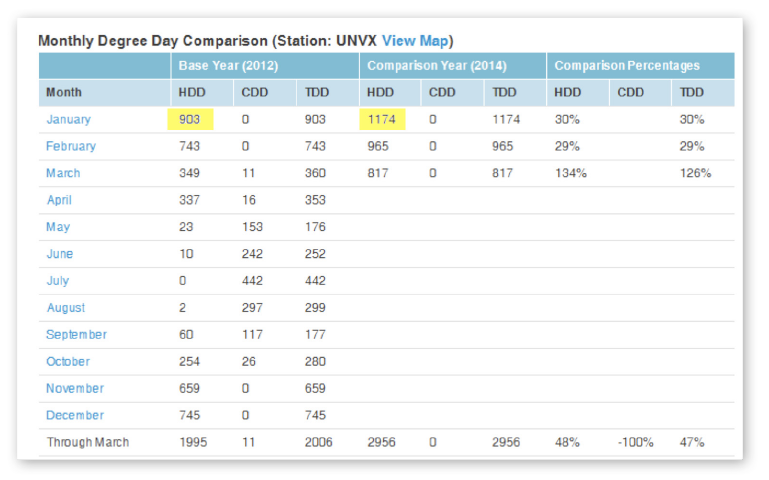
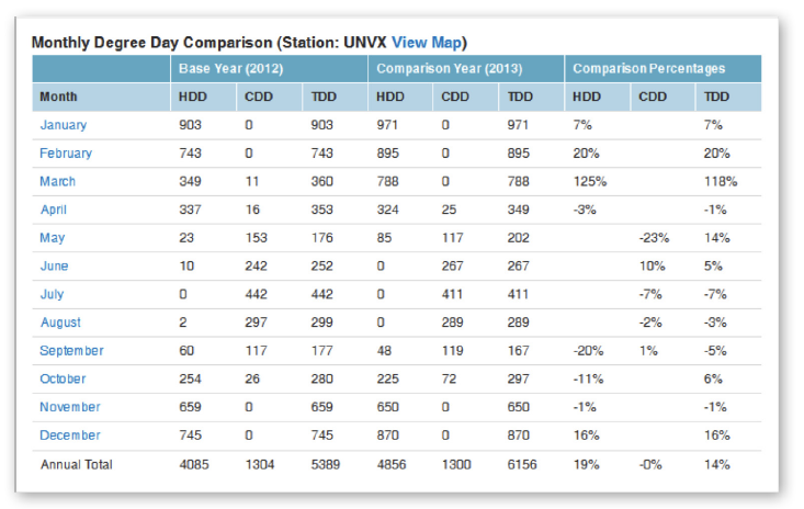
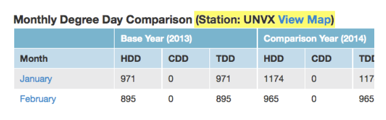
Below is a chart from WeatherDataDepot.com, comparing heating and cooling degree days in a base year (2012) with partial data from the current comparison year (2014). Degree days provide a metric for weather severity.
As you can see from the chart data, weather for the first three months of 2014 was more severe than the comparison year. In January 2012, for example, there were 903 heating degree days (HDD). By contrast, in January 2014, 1174 heating degree days were recorded for that location.
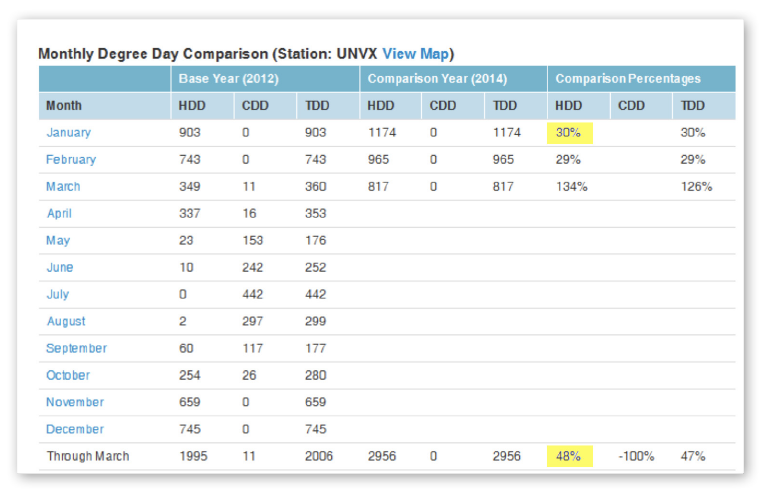
The comparison percentage columns reveal that this difference represents a 30 percent increase in weather severity. When we look at the three-month average (Jan–Mar), we see a 48 percent increase in weather severity, expressed as heating degree days, from the base year.
Combining this information with the CBECS weather data, it is now possible to calculate a reasonable value for budget impact:
Weather Load = 43 percent of energy expense
Comparison Year = 48 percent rise
The following formula calculates the percentage increase in energy expense:
0.43 * 0.48 = 20.64 percent
This example illustrates that weather has a significant impact on organization energy expenses. It also demonstrates how easy it is to analyze that impact when the data is available.
Degree Days
Previously we discussed degree days as a measure of weather severity. Let’s explore degree days in more detail.
Degree days represent the only weather metric that is consistently used in the context of building energy use. Heating degree days represent a need for heating to maintain a comfortable temperature in a building. Cooling degree days represent a need for cooling to maintain a comfortable temperature in a building. But how are degree days calculated?
Determining a Balance Point
The first step is to determine a consistent balance point temperature. This is the point at which a building requires neither heating nor cooling. The balance point for a specific building can vary greatly from a norm/average, depending on a number of factors including construction materials, insulation, date of construction, and more. Typically values from 55 to 65° F are chosen. EnergyCAP energy management software uses a linear regression analysis to determine the weather sensitivity of a given gas or electric meter using utility bill information and degree day data. By discarding outlier data points, a ‘best-fit’ line can pinpoint the ideal balance point on a meter-by-meter basis.
After the balance point temperature has been selected, daily degree day totals are calculated by obtaining the mean daily temperature for the building location and comparing that value to the building balance point.
For example, let’s suppose that you’re using a balance point of 60° F for a building, and the mean daily temperature for that location on January 1, 2014, is 30 degrees. To determine the number of heating degree days for that date, it is necessary to compare the mean daily temperature value with the balance point. This comparison reveals that there were 30 heating degree days on January 1, 2014 (60-30=30).
A key to grasping the degree day concept is to realize the importance of tracking daily heating and cooling values separately. If you attempt to simply calculate the average temperature on a weekly, monthly, or annual basis, contrasting heating and cooling data points would cancel each other out, especially in the “swing” seasons of spring and fall.
It has already been noted that, a linear regression can be performed from known weather and meter energy data to determine the optimum balance point on a building-by-building basis (assuming building-level metering). However, not all analysis is based on the optimum balance point. For instance, if you access a website database such as the National Weather Service, you will often spot a 65° F balance point. The 65° F balance point was established as the reporting standard in the 1930s when the degree day concept was first developed. It was based on daily dry bulb temperature and gas consumption data available for natural gas-heated residences during that period.
Commercial buildings and many institutional buildings today have a much lower balance point. There are a number of reasons for this. The envelope of these buildings is insulated better. There are many more internal heat gains due to equipment and lighting and plug load than would have been present in residences in 1930. So a 65-degree balance point is not really a defensible standard.
WeatherDataDepot.com enables the user to set any desire balance point. The default setting is 60.
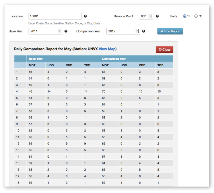
Here are two exercises to clarify the degree day concept. They are based on the chart data below:
QUESTION: Assume a balance point of 60° F. Assume a mean daily temperature (MDT) on May 1 of 56° F in the base year (2011). What is the degree day value for May 1?
ANSWER: The difference between the balance point temperature and the mean daily temperature is 4. Because the MDT is cooler than the balance point, heating would be required, so the value represents heating degree days.
QUESTION: Assume a balance point of 60° F. Assume an MDT on May 12 of 69° F in the base year (2011). What is the degree day value for May 12?
ANSWER: The difference between the balance point temperature and the mean daily temperature is 9. Because the MDT is warmer than the balance point, cooling would be required, so the value represents cooling degree days.
As the chart indicates, a degree day value is determined for each day of the month. Each day it is possible to have heating degree days or cooling degree days, or none (MDT = building balance point). But you will never see both heating and cooling degree day values for the same day.
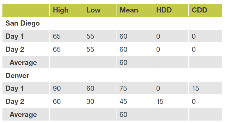
As long as the heating degree days and the cooling degree days are calculated independently, they represent an excellent measure of weather severity. The problem some people encounter is when they attempt to aggregate the two by combining and/or averaging the values. To see why this doesn’t work, consider two cities: San Diego, CA, and Denver, CO. And consider two days:
In San Diego, the mean daily temperature on both days was 60° F, which is fairly typical for San Diego.
By contrast, Denver’s temperatures were quite different. The first day was very hot, with a high of 90° and a low of 60°, producing an MDT of 75° F for 15 cooling degree days. On day two, a cold front from the western mountains blew through, producing a high temperature of 60° F and a low temperature of 30° F, producing an MDT of 45° F for 15 heating degree days.
If we try to aggregate the two-day data for both cities by considering only the MDT rather than the degree day values, we “discover” that their weather was identical. The two-day MDT average is 60° F. The faulty aggregation process has smoothed out the disparate weather data and rendered it meaningless!
In actuality, the energy required to maintain building temperatures in Denver on those two days was much greater than in San Diego. Only the degree day concept enables us to accurately assess the difference in weather severity.
The same principal holds true when considering aggregate annual temperature data. The average annual MDT for San Diego is 65° F. So is Dallas, TX. But in Dallas, people spend much more money on air conditioning in the summer and heating in the winter.
Accurately Analyzing Weather Trends
Now let us examine how we can use six Weather Data Depot functions to accurately analyze weather trends.
1. Monthly Degree Day Comparisons: Earlier we saw how easy it was to compare a base year with a comparison year. A positive comparison percentage means that the weather in the comparison year was harsher (more degree days). A negative percentage means that the weather in the comparison year was milder (fewer degree days). In a mild year, less energy would be required for heating or cooling.
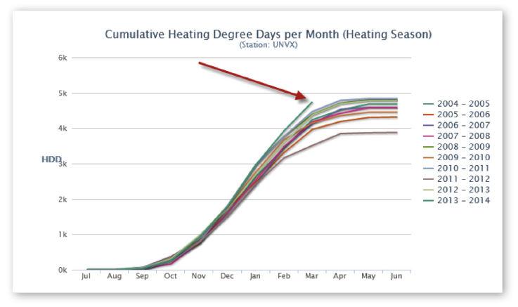
2. Cooling and Heating Cumulative Trends: WeatherDataDepot.com also provides a multi-year 12-month graph presenting annual cooling and heating cumulative trends. The chart below is plotting ten years of cumulative heating degree days. Each line represents a full year of monthly degree day data. The monthly data is aggregated from daily degree day data. It is also possible to view the same chart with cooling degree day data.
Since the graph is cumulative, each month’s degree total is added to the month before. This sort of metadata can be quite useful in budgeting and forecasting.
The chart illustrates that the temperature during the 2013–2014 heating season has been much more severe for this location than any year in the past ten years. That’s a nice piece of information to have when you’re trying to explain to the controller or the CFO why your utility bills are higher.
The curve of the chart data also enables a quick assessment of weather severity. In San Diego, the cumulative temperature curves would be much flatter since there are fewer seasonal variations and the region is more temperate.
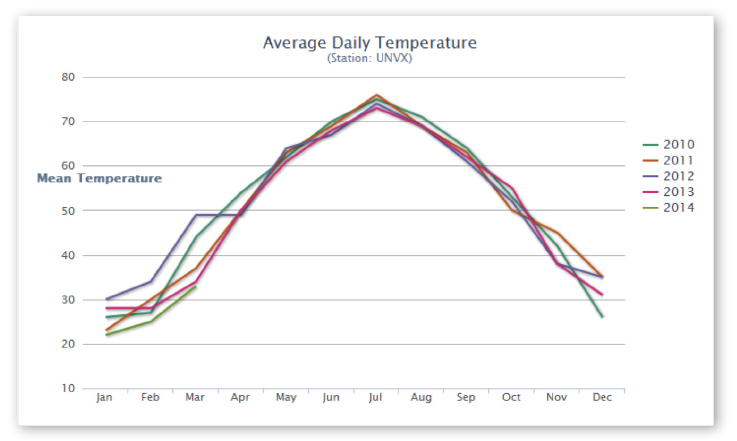
3. Monthly Trends: In addition to the cumulative graphs, there are also monthly trend line graphs on WeatherDataDepot.com. The chart below provides monthly mean temperature weather data for five years. Each year of monthly temperature data points is represented by a different-colored line.
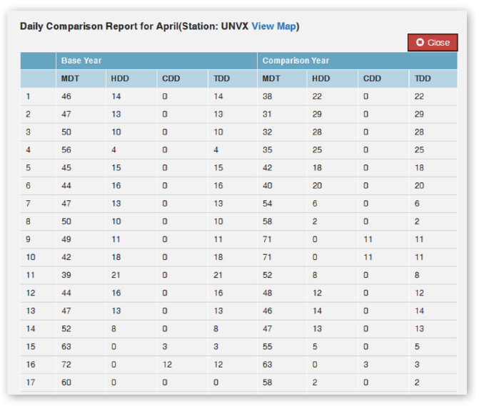
4. Daily Degree Day Data: Another advantage of WeatherDataDepot.com is the ability to “drill down” to the daily degree day data on which the monthly HDD and CDD totals are based.
To view the daily degree days for your location, click the hyperlink for the desired month from the Monthly Degree Day Comparison chart:
After you have selected the desired month, you will see a similar table with the days of the month indicated in the leftmost column:
5. Copy to Clipboard: All the charts on WeatherDataDepot.com are presented with a corresponding data table. The “Copy to Clipboard” button copies the data table to your Windows Clipboard.
From there, you can cut and paste in Excel to further manipulate the data for custom reports and alternative presentations.
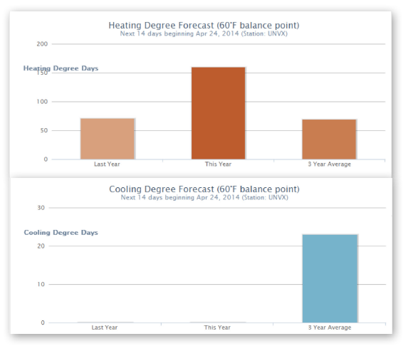
6. Degree Day Forecasting: WeatherDataDepot.com provides a unique forecasting feature. Each morning, a new degree day forecast is released looking two weeks into the future (a full 14 days).
The charts provide separate heating and cooling degree day forecasts, comparing this year’s forecast with actual data for last year and a bonus comparison with the average actual degree day values from the last three years.
Questions and Answers
WeatherDataDepot.com also includes an extensive FAQ page, answering questions like “How do we calculate degree days?” Or “Why does temperature data sometimes vary from one source of data to another source?”
The FAQ page also includes a download link for an Excel document containing all the weather locations managed by TWC. The file includes the official (long) title for the station, as well as its elevation. Elevation is particularly helpful if you are choosing between two local stations for presenting your weather data, since changes in elevation can lead to significant differences in degree day values.
The View Map link from the Monthly Degree Day Comparison Chart on WeatherDataDepot.com links to a Google map showing the area represented by the weather station. Keep in mind, however, that if you explore the circle defined by the Google map, you may not be able to discover an actual, physical, weather station.
Although there are hundreds of physical weather stations in the list, the bulk of them are virtual stations. They are created by TWC, using a computer simulation that interpolates data between actual ground stations and satellite data, as well as the National Weather Service and various other sources.
People often wonder about the accuracy of temperature modeling without accounting for variables such as humidity, cloud cover, wind velocity. Don’t those have an impact on building energy consumption as well? And why doesn’t WeatherDataDepot.com (and other sources) take that information into account? There are a few reasons:
1. Cost of Data: There is a huge increase in the cost of data for these multiple data points. Dry bulb temperature for MDT is the cheapest and easiest to obtain, and is an acceptably accurate predictor of building energy use.
2. Increased computational complexity: Multiple data points multiply the complexity of data processing and correlation. This can lead to potentially significant errors. And getting additional data becomes much more expensive.
3. Lack of Reliable Data: Once you say, “I also want to take humidity and wind into account,” then the available data quickly becomes scanty. By contrast, historical reliable dry bulb temperature is available as far back in time as 1995.
4. Studies Don’t Show A Benefit: We do have good historical data back to 1995 for dry bulb temperature, but not for some of the other variables. Most importantly, various studies have demonstrated that there is not a statistically significant analytical improvement when additional factors are taken into account.
Now someone might say, “Wait a second. I’m a mechanical engineer. I know that humidity affects the energy usage of my building. I know wind velocity is responsible for the wind chill effect and it affects the heat loss in my building.” And yes, that’s very true on a day-to-day basis. But the primary use of degree day data is for month-to-month and year-to-year comparisons. And what we find over these longer periods is that the humidity, the cloud cover, and the wind velocity does not change very much from year to year.
We also find a high degree of cross-correlation between dry bulb temperature and these other factors. In the end, when you look at the variables from a statistical standpoint and from a heat loss standpoint—energy transfer from the envelope of a building and so on—the bottom line is that accounting for these additional variables does not provide a significant analytical benefit. The extra data just does not really help us very much and it is more expensive, much harder to acquire and integrate, and a great deal harder to understand. In nearly every situation, the level of precision provided by dry bulb and degree day measurements is entirely sufficient.
Conclusion
The correlation between weather and energy use for many building types can be estimated using the CBECS survey tool. It can also be quantified using available energy data from your utility bills, coupled with publicly-available heating and cooling degree day weather data. WeatherDataDepot.com is an excellent resource for historical degree day information. Once the weather impact for a building’s energy consumption is known, that knowledge can aid in budgeting, forecasting, and trend analysis.
<?
/******************************************************
TOP BOX HEADLINE
******************************************************/
?>
This website stores cookies on your computer. These cookies are used to collect information about how you interact with our website and allow us to remember you. We use this information in order to improve and customize your browsing experience and for analytics and metrics about our visitors both on this website and other media. For more information, read our Privacy Policy.
Functional
Always active
The technical storage or access is strictly necessary for the legitimate purpose of enabling the use of a specific service explicitly requested by the subscriber or user, or for the sole purpose of carrying out the transmission of a communication over an electronic communications network.
Preferences
The technical storage or access is necessary for the legitimate purpose of storing preferences that are not requested by the subscriber or user.
Statistics
The technical storage or access that is used exclusively for statistical purposes.The technical storage or access that is used exclusively for anonymous statistical purposes. Without a subpoena, voluntary compliance on the part of your Internet Service Provider, or additional records from a third party, information stored or retrieved for this purpose alone cannot usually be used to identify you.
Marketing
The technical storage or access is required to create user profiles to send advertising, or to track the user on a website or across several websites for similar marketing purposes.

 Best-in-class portfolio-level energy and utility bill data management and reporting.
  Real-time energy and sustainability analytics for high-performance, net-zero buildings.
  A holistic view of financial-grade scope 1, 2, and 3 carbon emissions data across your entire business.
  Energy and sustainability benchmarking compliance software designed for utilities.